Linear Regression (with gradient derivation and Pyscript demo)
Published:
Introduction
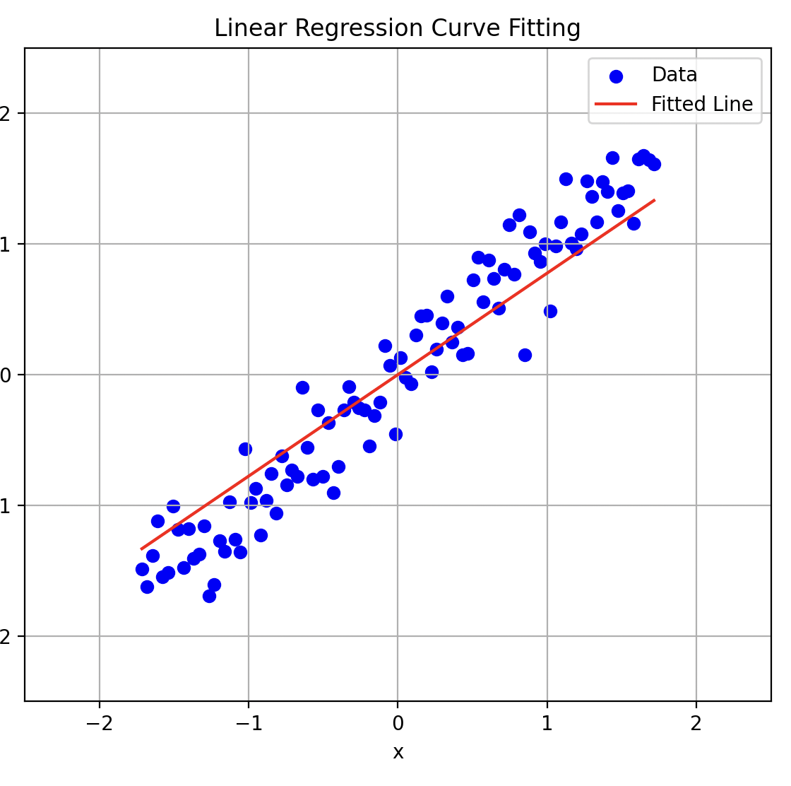
Linear regression models the relationship between a dependent variable \(y\) and independent variables \(X\) as a linear function. It finds coefficients \(\beta\) that minimize the error between predicted and actual values.
Mathematical Formulation
The dataset is labelled, \((\mathbf X, \mathbf y)\), and is assumed to follow this equation:
\[\mathbf{y} = \mathbf{X\mathbf W } + \mathbf b + \mathbf \epsilon\]Where:
- \(\mathbf{y} \in \mathbb{R}^{m}\): Target vector (\(m\) is the number of samples)
- \(\mathbf{X} \in \mathbb{R}^{m \times d}\): Feature matrix with \(d\) features (including a column of ones for the intercept)
- \(\mathbf{b}\in \mathbb{R}^{m}\): Bias vector
- \(\mathbf W \in \mathbb{R}^{d}\): Coefficients vector
- \(\boldsymbol \epsilon \sim \mathcal{N}(0, \sigma^2 \mathbf I)\in \mathbb{R}^{m}\): Error term (Gaussian noise with variance \(\sigma^2\) )
The model is given by
\[\hat{\mathbf{y}} = \mathbf{X} \mathbf{W} + \mathbf{b}\]Training
The cost function is MSE (Mean Squared Error), with L2 regularization (ridge regression)
\[J(\mathbf{W}, \mathbf{b}) = \frac{1}{2m} \|\mathbf{X} \mathbf{W} + \mathbf{b} - \mathbf{y}\|^2 + \frac{\lambda}{2} \|\mathbf{W}\|^2\]1. Gradient Equations
The gradients with respect to \(\mathbf{W}\) and \(\mathbf{b}\) are derived as follows:
Gradient with Respect to \(\mathbf{W}\):
\[\nabla_{\mathbf{W}} J(\mathbf{W}, \mathbf{b}) = \frac{1}{m} \mathbf{X}^\top (\mathbf{X} \mathbf{W} + \mathbf{b} - \mathbf{y}) + \lambda \mathbf{W}\]Gradient with Respect to \(\mathbf{b}\):
\[\nabla_{\mathbf{b}} J(\mathbf{W}, \mathbf{b}) = \frac{1}{m} \sum_{i=1}^m (\mathbf{X} \mathbf{W} + \mathbf{b} - \mathbf{y}) = \frac{1}{m} \mathbf{1}^\top (\mathbf{X} \mathbf{W} + \mathbf{b} - \mathbf{y})\]where \(\mathbf{1}\) is a vector of ones.
Note \(\mathbf{b}\) does not appear in the regularization term:
The updates for \(\mathbf{W}\) and \(\mathbf{b}\) are:
\[\mathbf{W} = \mathbf{W} - \alpha \nabla_{\mathbf{W}} J(\mathbf{W}, \mathbf{b})\] \[\mathbf{b} = \mathbf{b} - \alpha \nabla_{\mathbf{b}} J(\mathbf{W}, \mathbf{b})\]2. Closed-Form Solution with Bias
To solve for \(\mathbf{W}\) and \(\mathbf{b}\) in closed form, we modify the design matrix \(\mathbf{X}\) to include a column of ones to represent the bias:
\[\tilde{\mathbf{X}} = \begin{bmatrix} \mathbf{X} & \mathbf{1} \end{bmatrix}, \quad \tilde{\mathbf{W}} = \begin{bmatrix} \mathbf{W} \\ \mathbf{b} \end{bmatrix}\]The cost function becomes:
\[J(\tilde{\mathbf{W}}) = \frac{1}{2m} \|\tilde{\mathbf{X}} \tilde{\mathbf{W}} - \mathbf{y}\|^2 + \frac{\lambda}{2} \|\mathbf{W}\|^2\]In this case, the regularization applies only to \(\mathbf{W}\) (excluding \(\mathbf{b}\)). This is achieved by constructing a block matrix for the regularization:
\[\tilde{\mathbf{R}} = \begin{bmatrix} \lambda \mathbf{I} & \mathbf{0} \\ \mathbf{0}^\top & 0 \end{bmatrix}\]The closed-form solution becomes:
\[\tilde{\mathbf{W}} = (\tilde{\mathbf{X}}^\top \tilde{\mathbf{X}} + \tilde{\mathbf{R}})^{-1} \tilde{\mathbf{X}}^\top \mathbf{y}\]Expanding \(\tilde{\mathbf{W}}\) gives:
\[\mathbf{W} = \left( \mathbf{X}^\top \mathbf{X} + \lambda \mathbf{I} \right)^{-1} \mathbf{X}^\top (\mathbf{y} - \mathbf{b})\] \[\mathbf{b} = \frac{1}{m} \sum_{i=1}^m \left(\mathbf{y} - \mathbf{X} \mathbf{W} \right)\]The regularization term applies only to \(\mathbf{W}\), not \(b\). Define the regularization matrix \(\tilde{\mathbf{I}}\):
\[\tilde{\mathbf{I}} = \begin{bmatrix} \mathbf{I} & \mathbf{0} \\ \mathbf{0}^\top & 0 \end{bmatrix}\]The regularized cost function becomes:
\[J(\tilde{\mathbf{W}}) = \frac{1}{2m} \|\tilde{\mathbf{X}} \tilde{\mathbf{W}} - \mathbf{y}\|^2 + \frac{\lambda}{2} \tilde{\mathbf{W}}^\top \tilde{\mathbf{I}} \tilde{\mathbf{W}}\]Set the gradient of \(J(\tilde{\mathbf{W}})\) with respect to \(\tilde{\mathbf{W}}\) to zero:
\[\frac{\partial J}{\partial \tilde{\mathbf{W}}} = \frac{1}{m} \tilde{\mathbf{X}}^\top (\tilde{\mathbf{X}} \tilde{\mathbf{W}} - \mathbf{y}) + \lambda \tilde{\mathbf{I}} \tilde{\mathbf{W}} = 0\]Simplify:
\[\tilde{\mathbf{X}}^\top \tilde{\mathbf{X}} \tilde{\mathbf{W}} - \tilde{\mathbf{X}}^\top \mathbf{y} + m \lambda \tilde{\mathbf{I}} \tilde{\mathbf{W}} = 0\]Rearrange:
\[(\tilde{\mathbf{X}}^\top \tilde{\mathbf{X}} + m \lambda \tilde{\mathbf{I}}) \tilde{\mathbf{W}} = \tilde{\mathbf{X}}^\top \mathbf{y}\]Solve for \(\tilde{\mathbf{W}}\):
\[\tilde{\mathbf{W}} = (\tilde{\mathbf{X}}^\top \tilde{\mathbf{X}} + m \lambda \tilde{\mathbf{I}})^{-1} \tilde{\mathbf{X}}^\top \mathbf{y}\]This gives the closed-form solution, including both \(\mathbf{W}\) and \(\mathbf b\).
Python Implementation
Note: only implement gradient descent training, not closed form solution